Introduction

Quantization is a commonly used acceleration technique in NN inference. The primary computational workloads in NNs come from Convolution, Linear Layers, and Attention, which are implemented by GEMM in the lower level. This blog aims to discuss the principles of quantization from the matrix multiplication perspective and to explain why some quantization methods are impractical. It also aims to review several LLM quantization methods from this perspective.

I define practical quantization as follows:

  1. Operation can still be performed using GEMM after quantization. This requires both mathematical feasibility and hardware support. It is a fundamental requirement for achieving acceleration.
  2. Quantization must lead to actual acceleration. Acceleration can arise from higher INT8 hardware throughput, or from the memory bandwidth saved by smaller memory footprint. Importantly, the benefits of acceleration must outweigh the quantization overhead.

Let’s do some math

Suppose an operator can be expressed in the form of matrix multiplication:
$$\mathbf{Y}=\mathbf{X} \mathbf{W}^\top,$$
where $\mathbf{X} \in \mathbb{R}^{N \times C}$, $\mathbf{Y} \in \mathbb{R}^{N \times D}$, $\mathbf{W} \in \mathbb{R}^{D \times C}$, while their quantized versions are denoted as $\hat{\mathbf{X}}$, $\hat{\mathbf{Y}}$, $\hat{\mathbf{W}}$. Our goal is to ensure that operations can still be performed using GEMM after quantization, i.e.:
$$\hat{\mathbf{Y}}=\hat{\mathbf{X}} \hat{\mathbf{W}}^\top.$$

Let the per-element quantization functions for $\mathbf{X}$, $\mathbf{Y}$, and $\mathbf{W}$ be denoted as $p_{nc}(\cdot)$, $q_{nd}(\cdot)$, $r_{dc}(\cdot)$ respectively:
$$\begin{aligned}
\hat{x}_ {nc} &= p_ {nc}(x_{nc}), \\
\hat{y}_ {nd} &= q_ {nd}(y_{nd}), \\
\hat{w}_ {dc} &= r_ {dc}(w_{dc}).
\end{aligned}$$
The corresponding dequantization functions are denoted as $p_ {nc}^{-1}(\cdot)$, $q_ {nd}^{-1}(\cdot)$, $r_ {dc}^{-1}(\cdot)$, i.e.:
$$\begin{aligned}
y_ {nd}
&= \sum_ {c=1}^{C} x_ {nc} w_ {dc}, \\
q_ {nd}^{-1}(\hat{y}_ {nd}) &= \sum_ {c=1}^{C} p_ {nc}^{-1}(\hat{x}_ {nc}) \cdot r_ {dc}^{-1}(\hat{w}_ {dc}).
\end{aligned}$$
The above formulas set the basic constraints that practical quantization should satisfy mathematically.

Some basic quantization methods

With this basic constraints, we can now discuss several fundamental quantization methods, including per-element, per-channel, per-token, and per-tensor quantization.

Per-element and Per-channel

In the basic constraints mentioned above, the dequantization function $q_ {nd}^{-1}(\cdot)$ on the left-hand side does not depend on $c$. Clearly, if the right-hand side quantization functions $p_ {nc}^{-1}(\cdot)$ and $r_ {dc}^{-1}(\cdot)$ depend on $c$, this constraint will be violated. This implies that these two conditions cannot be satisfied at the same time:

  1. Computation can be done by GEMM.
  2. Different quantization functions can be applied in different channels of $\mathbf{X}$ and $\mathbf{W}$.

In other words, this indicates that per-element and per-channel quantization cannot be accelerated using GEMM. They are impractical.

Per-token and per-tensor

From the above discussion, we know that practical quantization needs to satisfy at least:
$$\begin{aligned}
p_ {n}(\cdot) &= p_ {nc} (\cdot), \quad \forall n, c, \\
r_ {d}(\cdot) &= r_ {dc} (\cdot), \quad \forall d, c.
\end{aligned}$$
That is, the quantization function is same for all channels. Therefore, the basic constraint can be formulated as:
$$q_ {nd}^{-1}(\hat{y}_ {nd}) = \sum_ {c=1}^{C_ i} p_ {n}^{-1}(\hat{x}_ {nc}) \cdot r_ {d}^{-1}(\hat{w}_ {dc}),$$
Thus, we get per-channel quantization. If we further assume:
$$\begin{aligned}
p(\cdot) &= p_ {nc} (\cdot), \quad \forall n, c, \\
r(\cdot) &= r_ {dc} (\cdot), \quad \forall d, c.
\end{aligned}$$
That is, the quantization function is same for all elements in both $\mathbf{X}$ and $\mathbf{W}$. Therefore, the basic constraint can be formulated as:
$$q_ {nd}^{-1}(\hat{y}_ {nd}) = q^{-1}(\hat{y}_ {nd}) = \sum_ {c=1}^{C_i} p^{-1}(\hat{x}_ {nc}) \cdot r^{-1}(\hat{w}_ {dc}).$$
We thus obtain per-tensor quantization. While both of these quantization methods have theoretical feasibility, the practical values of them are still limited by hardware support (as discussed in the next section).

For convenience, the following discussion focuses only on per-token quantization. Per-tensor quantization can be seen as a special case of per-token quantization. The most commonly used quantization method in practice is symmetric uniform quantization, which scales the value range using multiplication, i.e.:
$$\begin{aligned}
\hat{x}_ {nc} &= p_ {n}(x_ {nc}) = p_ n x_ {nc}, \\
\hat{w}_ {nd} &= r_ {d}(w_ {dc}) = r_ d w_ {dc}, \\
\hat{y}_ {dc} &= q_ {nd}(y_ {nd}) = p_ n r_ d y_ {nd}.
\end{aligned}$$

We can formulate per-token symmetric uniform quantization by matrix multiplication:
$$\begin{aligned}
\hat{\mathbf{X}} &= \text{diag}(p_1,\cdots,p_ N)\cdot \mathbf{X} = \begin{pmatrix}
p_ 1 & \cdots & p_ 1 \\
\vdots & \ddots & \vdots \\
p_ N & \cdots & p_ N
\end{pmatrix} \otimes \mathbf{X}, \\
\hat{\mathbf{W}} &= \text{diag}(r_1,\cdots,r_ D)\cdot \mathbf{W} = \begin{pmatrix}
r_ 1 & \cdots & r_ D \\
\vdots & \ddots & \vdots \\
r_ 1 & \cdots & r_ D
\end{pmatrix} \otimes \mathbf{W}, \\
\hat{\mathbf{Y}} &= \text{diag}(p_1,\cdots,p_ N)\cdot \mathbf{Y} \cdot \text{diag}(r_1,\cdots,r_ D) = \begin{pmatrix}
p_ 1 r_ 1 & \cdots & p_ 1 r_ D \\
\vdots & \ddots & \vdots \\
p_ N r_ 1 & \cdots & p_ N r_ D
\end{pmatrix} \otimes \mathbf{Y},
\end{aligned}$$
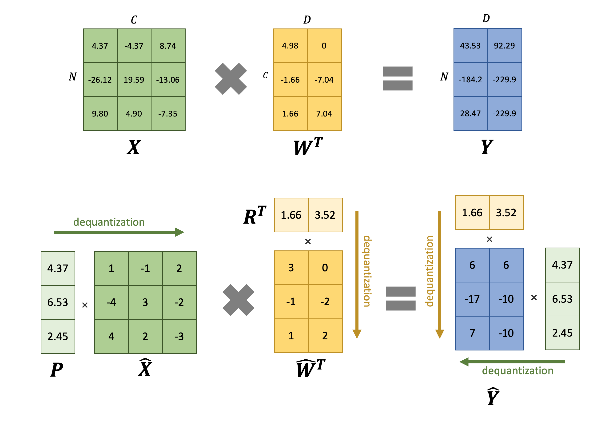
where $\otimes$ represents element-wise matrix multiplication. It can be observed that both quantization and dequantization can be efficiently implemented using element-wise matrix multiplication with dimension broadcasting. The following figure illustrates the computation process by an example:

Hardware requirements

Hardware support still need to be considered when we try to utilize GEMM for quantization. For example, on NVIDIA GPUs, Tensor Core supports matrix multiplication for FP16 and INT8, but it doesn’t support mixed precision matrix multiplication for FP16/INT8. This means that W8A8 quantization can benefit from Tensor Core, but W8A16 and W16A8 quantization lack hardware support and may not achieve real acceleration on NVIDIA GPUs. Many W8A16 and W16A8 quantization methods actually perform dequantization before GEMM and then use FP16 for computation. The actual acceleration effects of these methods require further discussion (see below).

Performance analysis

The above discussion only shows that per-token quantization can leverage GEMM. The following words will show whether it can provide actual acceleration.

We compare the following three setups:

  1. Unquantized, using FP16 for both storage and computation.
  2. W8A8 quantization, with I/O activations stored in FP16. This is the approach used by some works like LLM.int8(). To avoid additional CUDA kernel launch overhead, we assume that quantization and dequantization are fused with GEMM.
  3. W8A16 quantization, internally converting weights to FP16 for computation. Kernel fusion is also applied here.

Without loss of generality, we can assume that the hardware INT8 throughput is $2\times$ than that of FP16. We can set normalized operations of one INT8 operation is $1$, while $2$ for FP16. We can list the following table:

Method FP16 W8A8 (FP16 activations I/O) W8A16
GEMM OPs $2NCD$ $NCD$ $2NCD$
GEMM mem I/O $2(NC+CD+ND)$ $2NC+CD+2N D$ $2NC+CD+2ND$
quant/dequant OPs $0$ $2NC+4ND$ $2CD$
quant/dequant Mem I/O $0$ $2(N+C_o)$ $2D$
total OPs $2NC D$ $NC D+2NC+4N D$ $2NCD+2CD$
total mem I/O $2(NC+C D+N D)$ $2NC+C D+2N D+2(N+C_o)$ $2NC+CD+2ND+2D$
total arithmetic intensity (OPs:I/O) $\cfrac{1}{1/N+1/C+1/D}$ $\cfrac{1+2/D+4/C}{2/N+1/C+2/D+2/(NC)+2/(CD)}$ $\cfrac{1+2/N}{1/(2N)+1/C+1/D+1/(NC)}$
total arithmetic intensity (second-order approximation) $\cfrac{1}{1/N+1/C+1/D}$ $\cfrac{1}{2/N+1/C+2/D}$ $\cfrac{1}{1/(2N)+1/C+1/D}$

Analyzing the table above, we can draw the following conclusions:

  1. W8A8 quantization (with FP16 activations I/O) reduces the operations by almost half compared to FP16, but it decreases the total arithmetic intensity. Therefore, in memory-bound scenarios, W8A8 quantization may not achieve a $2\times$ throughput improvement (ZeroQuant addresses this issue, as discussed below). But it can still lead to a significant throughput improvement when memory bandwidth is sufficient.
  2. W8A16 quantization maintains a similar operations compared to FP16, but it slightly increases the total arithmetic intensity (more increase when $N$ is large). Therefore, it also has practical value in memory-bound scenarios, especially since activations in LLMs are typically harder to be quantized than weights.

Some LLM Quantization works

LLM.int8()

LLM.int8() actually employs selective per-token quantization. It stores weights and activations in FP16 and then applies different strategies for different tokens, as illustrated below:

LLM.int8()

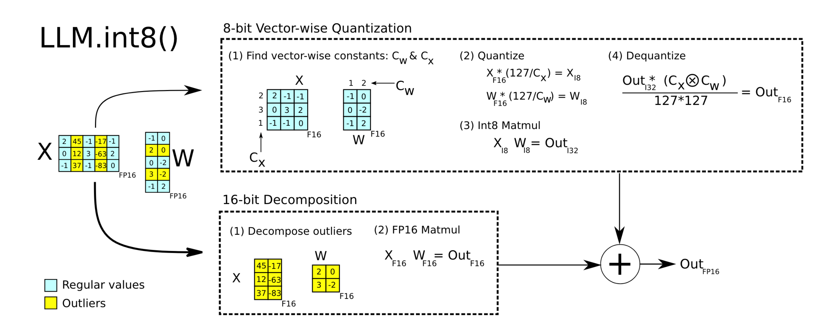
  • For tokens suitable for quantization, it applies per-token INT8 quantization to weights and activations, computes results using INT8 GEMM, and then dequantizes them to FP16.
  • For tokens with outliers, it directly computed the FP16 GEMM.

The results from these two parts can be combined to form the final result.

SmoothQuant

While per-channel quantization may not be practical, for LLM activation quantization, the main challenge arises from activations, where values with larger magnitudes may appear on some channels, as shown below:

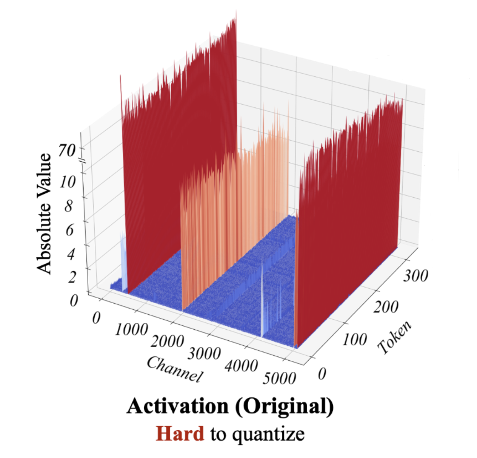
SmoothQuant observed that these outliers occur consistently in specific channels, while outliers are rare in weights (thus easier to quantize). Therefore, it proposes to “balance” the quantization difficulty between activations and weights by introducing a per-channel scaling factor:

SmoothQuant

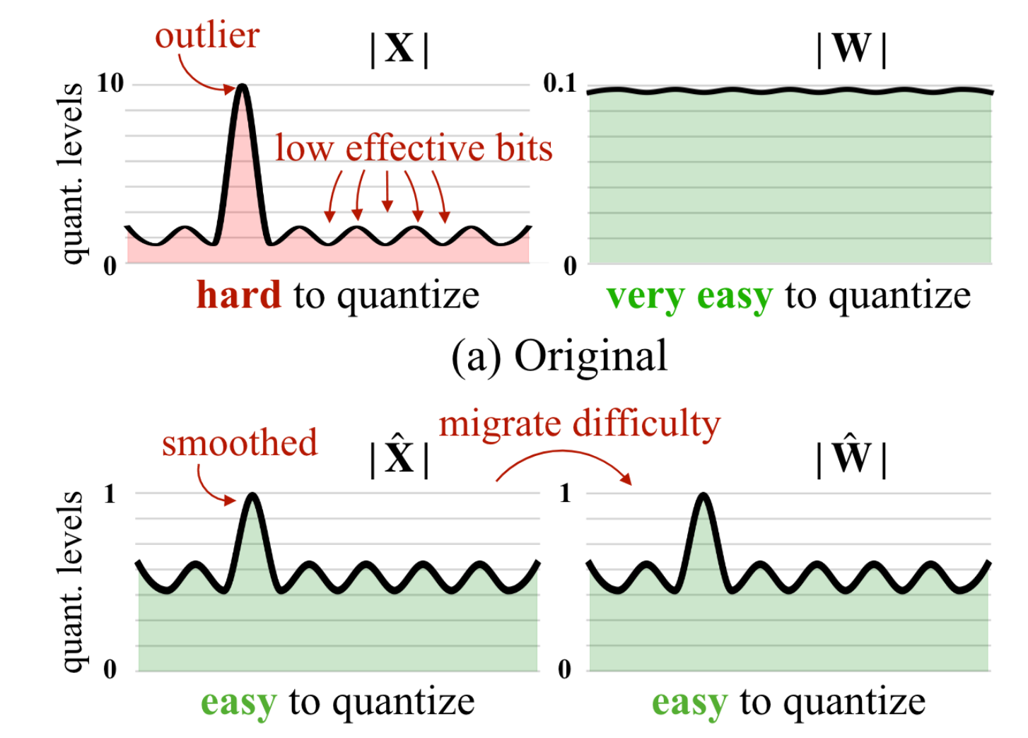
This “balance” can be formulated as:
$$\begin{aligned}
\mathbf{Y}
&= \mathbf{X}\mathbf{W}^\top \\
&= \mathbf{X} \cdot \text{diag}(s_ 1,\cdots,s_ C) \cdot \text{diag}(s_ 1,\cdots,s_ C)^{-1} \cdot \mathbf{W}^\top \\
& = \left( \mathbf{X} \cdot \text{diag}(s_ 1,\cdots,s_ C) \right) \cdot \left( \mathbf{W}\cdot \text{diag}(s_ 1,\cdots,s_ C)^{-1} \right)^\top.
\end{aligned}$$
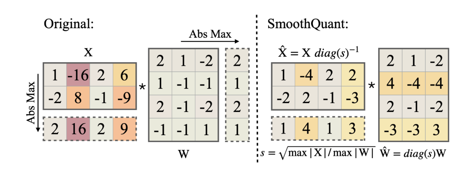
By selecting appropriate scaling factors $\text{diag}(s_ 1,\cdots,s_ C)$, we can achieve the goal of balancing outlier values in activations, and then we can quantize $\mathbf{X} \cdot \text{diag}(s_ 1,\cdots,s_ C)$ and $\mathbf{W}\cdot \text{diag}(s_ 1,\cdots,s_ C)^{-1}$. The following figure give an example:

SmoothQuant example

SmoothQuant is an excellent alternative to per-channel quantization, as demonstrated in the paper by its impressive performance in quantizing LLM to W8A8.

ZeroQuant

In the above performance analysis of W8A8, we found that using FP16 for activations I/O reduces the overall arithmetic intensity after quantization, which may harm the throughput improvement in memory-bound scenarios. ZeroQuant addresses this issue by fusing the quantization into the previous operator and fusing the dequantization after GEMM, as shown in the figure below.

ZeroQuant

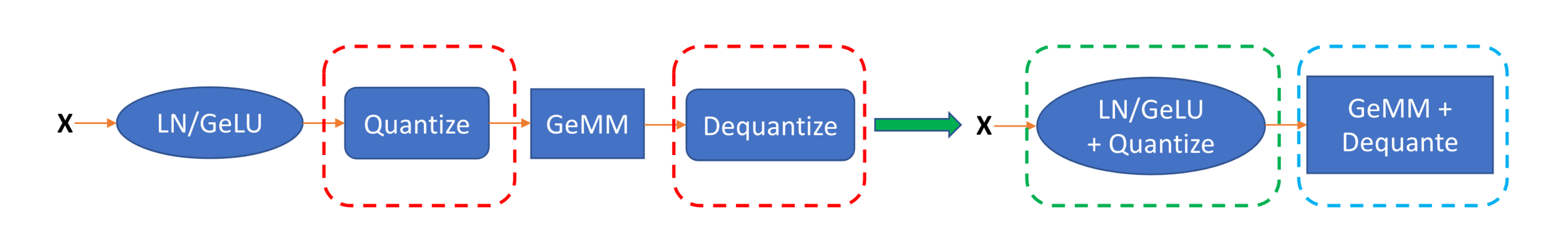
Thus, the activations I/O between operators are still INT8, which reduces the total memory I/O to $NC+CD+ND+2(N+D)$, boosting arithmetic intensity to original FP16 level , and fully leveraging the high throughput of INT8.

Conclusion

This blog provides a matrix multiplication perspective for quantization, indicating some fundamental requirements for practical quantization and explaining why per-channel quantization in impractical. It also discusses several examples of LLM per-token quantization, including LLM.int8(), SmoothQuant, and ZeroQuant.
They are all practical and demonstrate significant acceleration in real-world scenarios.

前言

本文是我在实践中总结出的生产场景下 10 Gbps 网络下的 NFS 性能调优指南,特别是针对大量小文件(Lots of Small Files, LOSF)读写的优化。

调优

硬件

网络硬件方面,带宽延迟两者都很重要。

要保证 NFS 的性能,高带宽网络是必要的,10 Gbps 对于生产场景来说是基础要求,更高速的 InfiniBand 或者 RoCE 网络则可按照需求和预算进行选择。

对于大量小文件(Lots of Small Files, LOSF)场景来说,延迟比带宽更重要。很多性能调优教程都忽略了这一点,只关注了连续读写的性能,即使测试了 4K 随机读写,也使用了错误的测试方法(下文给出了正确的测试方法)。

延迟的重要性体现在,如果程序对于小文件的访问是内秉串行化的,延迟会决定串行化 IOPS 的上限。0.1 ms 的延迟决定了串行化的 IOPS 上限是 10k,而 1 ms 的延迟对应的上限则是 1k。

内秉串行化访问的场景非常多。例如,把家目录放置于 NFS 上,oh-my-zsh 的加载、python 包的加载都是内秉串行化的。1ms 的网络延迟会让这些程序慢到不可接受(例如 import torch 的执行需要 30s 以上)。

使用合格的企业级交换机、恰当配置的网络拓扑,可以尽量降低延迟。同时,光模块、光转电口模块的质量也有可能极大影响延迟(我原来使用的中科光电光转电口模块会引入 0.1ms 的额外延迟,导致 IOPS 下降了 2/3)。

需要注意的是,RDMA 尽管理论上能降低延迟,但实际测试中发现 10 Gbps 以太网和 100 Gbps InfiniBand 的串行化 IOPS 差距并不大,预算有限时只使用以太网也足够。

TODO: 巨型帧

Linux Kernel

内核网络参数需要进行调整,以适应高速网络:

1
2
3
4
5
6
7
8
9
10
11
12
13
14
15
16
17
18
19
# Ref: https://gist.github.com/mizanRahman/40ba603759bfb5153189ccdc9dbbd1e4

# Disable TCP slow start on idle connections
net.ipv4.tcp_slow_start_after_idle = 0

# Increase Linux autotuning TCP buffer limits
# Set max to 16MB for 1GE and 32M (33554432) or 54M (56623104) for 10GE
# Don't set tcp_mem itself! Let the kernel scale it based on RAM.
net.core.rmem_max = 56623104
net.core.wmem_max = 56623104
net.core.rmem_default = 56623104
net.core.wmem_default = 56623104
net.core.optmem_max = 40960
net.ipv4.tcp_rmem = 4096 87380 56623104
net.ipv4.tcp_wmem = 4096 65536 56623104

# TCP Congestion Control
net.ipv4.tcp_congestion_control = bbr
net.core.default_qdisc = cake

在服务端和客户端都需要应用这套设置,可以写入 /etc/sysctl.conf 中以持久化。

Server Side

NFS server 的线程数可以尽量调大点,服务器负载比较高时可以提升性能,我直接设成了服务器的线程数。修改 /etc/nfs.conf

1
2
[nfsd]
threads=128

以下几个 NFS server 参数需要调整:

  • async:将同步 IO 操作视为异步。同步读写为主的负载可以大幅提升性能,但服务器崩溃时可能造成数据丢失,对数据完整性有极高要求的情况下不推荐使用;
  • no_subtree_check:对性能没有大影响,但在某些情况下可以提升可靠性(同时有轻微的安全风险)。参见 [1]。

Client Side

没有特殊的理由时应该默认使用最新的 NFSv4.2,NFSv3 使用 UDP 作为底层传输方式时,在高速网络下会因为 UDP 包序列号问题导致数据损坏,参见 [2]。

以下几个 NFS client 参数需要调整:

  • proto=rdma:网络支持 RDMA 时设置;
  • nocto:关闭 close-to-open 缓存一致性语义。NFS 默认行为是关闭文件时会把所有更改写回到服务器。如果对于多客户端之间的文件一致性要求比较高,不推荐使用此选项;
  • ac:启用属性缓存(attribute caching),客户端会缓存文件属性。同样。对于数据一致性要求较高的集群,不推荐使用此选项;
  • fsc:使用 FS-Cache 缓存数据到本地。需要同时配置 cachefilesd。奇怪的是我在测试中并没有发现数据被缓存到本地,这可能需要进一步的探究;
  • nconnect=16:设置 NFS client 和 server 间建立 16 条 TCP 连接。NFS client 默认只建立一条 TCP 连接,所有 RPC 复用这条连接。在某些情况下这会限制连续读写的带宽。增大 nconnect(最大值 16)可以解决这个问题。

特别的,noatime / relatime 的设置对于 NFS 并无影响 [3],NFS client 始终会缓存 atime 的更改。

有些教程中会推荐修改 rsizewsize,这两个值在 NFSv4.2 默认协商出的即是最大值 1048576,因而无需手动更改,只需检查一下是否协商正确即可。

根据 [4],sunrpc.tcp_max_slot_table_entries 可能会影响性能,可以适当调大(默认 2)。在我的测试中,我发现当遇到千万数量级的持续小文件访问负载时,NFS 有时候会卡住。当我把这个参数调大时,此问题得以解决。设置 /etc/modprobe.d/sunrpc.conf

1
options sunrpc tcp_slot_table_entries=16384

有时我会遇到 nfsd 占用大量 CPU 且性能急剧下降的问题,同时记录到大量 delegreturn RPC calls。根据 [5],可以通过禁用 fs.leases-enable 解决,设置 /etc/sysctl.conf

1
fs.leases-enable = 0

nfsd 因为种种原因重启后,默认会有 90s 的 grace period 用于锁恢复,这段时间内 nfsd 会拒绝所有 open 请求,在内核日志中显示:

1
[1073511.138061] NFSD: starting 90-second grace period (net f0000000)

实践中发现这段时间可以适当调小,以减少 nfsd 重启带来的影响。设置 /etc/default/nfs-kernel-server

1
2
# Options for rpc.svcgssd.
RPCSVCGSSDOPTS="--lease-time 10 --grace-time 10"

测试

TODO

总结

TODO

参考

[1] https://man.archlinux.org/man/exports.5.en#no_subtree_check

[2] https://man.archlinux.org/man/nfs.5.en#Using_NFS_over_UDP_on_high-speed_links

[3] https://man.archlinux.org/man/nfs.5.en#File_timestamp_maintenance

[4] https://learn.microsoft.com/en-us/azure/azure-netapp-files/performance-linux-concurrency-session-slots

[5] https://docs.gitlab.com/ee/administration/nfs.html#disable-nfs-server-delegation

This blog is a write-up of the paper “ACS: Concurrent Kernel Execution on Irregular, Input-Dependent Computational Graphs“ from arXiv’24.

Motivation

Some workloads (e.g., Simulation Engines for Deep RL, Dynamic DNNs) cannot fully utilize the massive parallelism of GPUs (see Figure 1). The main reason is that these workloads contain lots of small kernels which cannot fully utilize the GPU, and these kernels are not executed concurrently, although most of them are independent and in theory can be executed concurrently.

Figure 1. Achieved Occupancy of simulation engines (up) and dynamic DNN (down)

But there are some challenges to execute these kernels concurrently:

  1. Input-dependent kernel dependencies. For some workload, the the dependencies between kernels are only determined at runtime for each input. Constructing full computational graph and resolving dependencies before execution will introduce high latency (see Figure 2,average of 47% of overall execution time as the paper says).

Figure 2. DAG construction time as % of execution time

  1. Irregular kernel dependencies. Some workloads have irregular computational graphs. We can partitioned the computational graph of the workload into independent streams of kernels. But this would require fine-grained scheduling and synchronization, with large overhead (see Figure 3).

Figure 3. Kernel launch and synchronization overheads

Existed solutions:

  1. CUDA Graph and AMD ATMI. They allow users specify dependencies between different kernels as DAG, and can eliminate the synchronization and kernel launch overhead. But the DAG needs to be constructed in full before execution, which imakes them not suitable for dynamic kernel dependencies (such as Dynamic DNNs).

  2. Using events provided by the CUDA stream management API, which allows synchronization between kernels across streams through the cudaStreamWaitEvent API, without blocking the host. But approach still requires deriving dependencies between all kernels beforehand.

  3. Persistent threads (PT) can eliminate the scheduling and launch overheads, but are only effective when all kernels are homogeneous.

    PT is just like coroutine in some programming languages.

  4. CUDA dynamic parallelism (CDP) or AMD’s device enqueue (DE) enables parent kernels to launch child kernels, but , only allowing data dependencies between one parent and its children (so cannot be use to synchronize between multiple tasks).

Design

The goal of this paper is to design a framework that enables efficient concurrent execution of GPU kernels with:

  1. lightweight detection of inter-kernel dependencies at runtime,

  2. low overhead kernel scheduling and synchronization.

The key idea is to perform the dependence checking and scheduling within a small window of kernels at runtime similar to out-of-order instruction scheduling.

The authors proposed Automatic Concurrent Scheduling (ACS) as solution. The overall design of ACS-SW is shown in Figure 4. It contains three main functionalities:

Figure 4. ACS-SW Overview

  1. Determining inter-kernel dependencies. By checking for overlaps between read segments and write segments, we determine dependencies between kernels. For a wide range of commonly used kernels (e.g., matrix multiplication, convolution), we can infer the read and write segments from the input easily. But for some kernels, it’s impossible to determine the range of memory accessed statically because of the potential indirect memory accesses, so the authors just assume the entire GPU memory may be accessed.

    Memory regions written to/accessed by the kernel

    The authors use a kernel wrapper to finish the dependency detection. get_addresses() is called to get __read_segments__ and __write_segments__.

    1
    2
    3
    4
    5
    6
    7
    8
    9
    10
    11
    12
    13
    struct ACE_wrapper { 
    //list of read,write segments defined as
    //[{start_adr1,size1},{start_adr2,size2}..]
    list __read_segments__;
    list __write_segments__;
    // function which gets called at kernel
    // launch to populate read,write segments
    void get_addresses(
    dim3 blocks, dim3 threads, ...
    );
    // function declaration of the kernel
    static __global__ void kernel(...);
    };
  2. Tracking kernel state at runtime. The kernels in the window can be three states:

    1. Ready: kernels it is dependent on complete execution.
    2. Pending: upstream kernels are still pending or executing.
    3. Executing.

Kernels in the scheduling window with their state and corresponding upstream kernels

  1. Eliminating CPU synchronization overheads. See ACS-HW for more details.

ACS has two variants:

  1. ACS-SW: software-only implementation which emulates the out-of-order kernel scheduling mechanism.

  2. ACS-HW: hardware-facilitated implementation which is more efficient as it also alleviates synchronization overheads.

ACS-SW

Window Module

This module is to determining inter-kernel dependencies. It is implemented as a separate thread that manages the input FIFO queue and the scheduling window. The kernel state tracking is implemented in the hardware.

Scheduler Module

This module schedules and launches ready kernels for execution. It has fixed number of CUDA streams. Each stream contains only one kernel at any given time. Threads with empty streams poll the scheduling window for a ready kernel.

ACS-SW: The scheduler module

ACS-HW

ACS-SW incurs kernel synchronization and launch overheads because scheduler module launches a kernel in the CPU. ACS-HW solves these problems by a software-hardware co-design.

ACS-HW Overview

Software-side: maintains an input FIFO queue like ACS-SW, and a list of kernels in the GPU’s scheduling window, but it can be stale.

Hardware-side: the scheduling window and its management are implemented in hardware on the GPU side.

A key novelty in hardware design is two stage dependency detections. First, ACS use software to perform initial detection using stale kernel information (without frequent synchronize overhead), then utilizes hardware to correct outdated dependency information. This two-stage approach significantly reduces the hardware complexity.

ACS-HW Scheduler

Evaluation

  1. Baseline: cuDNN implementation (for DNNs) and a jax implementation (for deep RL simulation), both using CUDA streams.
  2. ACS-SW: on real hardware.
  3. ACS-SW-Sim: ACS-SW on the GPU simulator.
  4. ACS-HW: on the GPU simulator.
  5. CUDAGraph.

Deep RL physics simulations: Normalized Speedup

Deep RL physics simulations: Normalized Speedup on GPU simulator

Deep RL physics simulations: Achieved occupancy

Dynamic DNNs: Normalized speedup

Dynamic DNNs: Achieved occupancy

Static DNNs: Normalized speedup

Static DNNs: Achieved occupancy

Comments

Strengths

This paper focuses on the problem of low GPU utilization caused by the serial execution of numerous small CUDA kernels. I believe this paper effectively addresses this problem, particularly with the following innovative points that are impressive me:

  1. Out-of-order dependency detection and scheduling. Out-of-order (OoO) is a common technique in micro-architecture and software (e.g., hard disk I/O queue) designs. It’s an impressive and innovative idea to introduce OoO into this area to find the dynamic dependencies efficiently.

  2. A good trade-off. When I first read the Introduction section of the paper, I thought the read-write dependencies detection may be a difficulty task. To my knowledge, there aren’t reliable static binary memory access analysis techniques (otherwise, segmentation fault wouldn’t be a common problem). However, the authors made a good simplification and trade-off regarding this problem. For most common kernels, memory access areas can be inferred from input parameters. For the rest kernels, it can be assumed that they access the entire memory. Since few common operators occupy most of the execution time, this trade-off leads to significant performance improvements with a relatively low scheduling overhead. This innovation is my favorite aspect of this paper.

  3. Two-stage dependency detection in ACS-HW. While a complete hardware dependency detection approach is theoretically feasible, it could incur significant chip area costs (as we know, the re-order buffer in microprocessor carries large area). The authors proposed a two-stage software-hardware co-design dependency detection, significantly simplifying the difficulty of hardware design. It is a brilliant idea.

Weaknesses

This paper has some potential weaknesses:

  1. To each type of kernel, we must custom get_addresses function int the kernel wrapper. This weakness may limit the adoption of ACS.

  2. Deciding whether kernels should be executed concurrently requires considering more factors than just data dependencies. If there are resource conflict (e.g., memory bandwidth, shared memory size) between two large kernels, performance may degrade if they co-execute.

Improvements

I propose some potential improvements to this paper:

  1. In response to the first weakness mentioned above, I propose a profiling-rollback strategy to achieve safe automatic dependency detection. This strategy leverages the commonly used paging technique in OS virtual memory management: we can set a memory page as read-only or write-only. When a program is running, if a page fault is triggered, we can know that a read/write occurs. While I’m unsure if Nvidia GPUs provide APIs for user to control page tables, let’s assume such APIs exist. Given that many workloads are iterative (e.g., neural network training), we can profile the workload just one iteration, utilizing the aforementioned paging trick to record the memory access segments of each kernel. Obviously this may introduce some inaccuracies, we need a rollback strategy to ensure correct program execution. During runtime, we set known __write_segments__ as read-write, while other areas are set as read-only. Upon encountering a page fault, we detect an error and revert to the default strategy (assuming all memory areas will be read and wrote). With this strategy, we can eliminate the need of manual get_addresses function, and maximize the potential parallelism.

  2. Regarding the second weakness, I suggest adopting the method of GPUPool to determine which kernels are suitable for concurrent execution. A naive solution involves tracking the number of SMs each kernel occupies. When the SMs of a GPU are fully occupied, even if there are kernels in the ready state and available CUDA streams, no new kernels are scheduled.

This blog is a write-up of the paper “GPUPool: A Holistic Approach to Fine-Grained GPU Sharing in the Cloud“ from PACT’22.

Motivation

This paper focuses on the GPU sharing in cloud scenarios.

Currently, existing GPU sharing techniques can be categorized into 2 types:

  • Time-sharing means executing each concurrent VM on a full device in a round-robin fashion. Pros: Simple and mature. Cons: VMs could still under-utilize the hardware within each time slice.

  • Shape-sharing: split a device into partitions and allows multiple workloads to execute on different partitions simultaneously.

Space-sharing can be categorized into 2 types:

  • Coarse-grained assigns disjoint sets of streaming multiprocessors (SMs) and memory channels to concurrent workloads. For example, Nvidia MIG. Pros: offers great performance isolation among tenants of the same GPU. Cons: (i) resource under-utilization within each SM consisting of heterogeneous functional units (e.g., FP32, INT, FP64, Tensor Cores) meant for different workload types. (ii) inefficient memory bandwidth usage caused by the bursty nature of GPU memory traffic.

  • Fine-grained allows different workloads to co-run on the same SMs and request memory bandwidth flexibly, such as CUDA Stream and MPS. Pros: Better hardware utilization.

The key problem of GPU sharing in data center is performance unpredictability. It contains 2 key challenges:

  1. Mitigating interference. The amount of performance improvement from fine-grained sharing varies drastically depending on how compatible the concurrent workloads are in terms of resource usage. Also, the interference cannot be statically estimated. So, it is non-trivial to determine compatibility among a large number of incoming jobs in the cluster.

  2. Providing QoS guarantees.

Existing solutions:

  • Software-based: kernel slicing or a persistent thread model. Cons: high scheduling overhead.

  • Hardware-based: integrate sophisticated resource management logic into hardware to allocate resources for concurrent kernels. Cons: expensive and also inflexible.

Common problems of existing solutions:

  1. They do not concern with interference mitigation at the cluster level.

  2. They do not handle scenarios where incoming jobs must be distributed among multiple GPUs to satisfy QoS constraints.

Figure 1. Simulated system throughput of co-running `parb_spmv` and `rod_hotspot` at various TBs/SM settings

Problems of hardware TB scheduler which hinder the fine-grained sharing:

  1. It always attempts to launch as many thread blocks per SM (TBs/SM) for each kernel as allowed by the execution context storage constraints (e.g., registers, shared memory, thread slots). It leaves insufficient resources for concurrent kernels. As showed in Figure 1, if we can individually set the TBs/SM for each kernel, we may achieve a higher throughput.

  2. It only dispatches concurrent kernels onto SMs after the earlier arriving one completes launching all the thread blocks specified by the kernel grid size. This will force an almost serially execution of kernels in some scenarios.

GPU applications in the cloud fall into two main categories: latency-sensitive, and throughput-oriented. Throughput-oriented workloads are good candidates for hardware space-sharing. They have the following characteristics:

  1. Most workloads involve a large variety of kernels with different hardware resource utilization characteristics (e.g., CNN: compute-intensive, batch-norm: memory-intensive).

  2. Active SMs are underutilized in some resources (FP, tensor core, memory bandwidth).

  3. They typically repeatedly execute the same sequence of kernels (e.g., ML).

  4. Relaxed QoS Requirements.

Design

This paper proposed a hardware-software co-designed strategy to solve these challenges.

Hardware

This paper changes the default behavior of CUDA runtime to make it more suitable for fine-grained sharing:

  1. Allows CUDA runtime to program the TBs/SM setting as one of the kernel launch parameters. The value of TBs/SM is selected by the performance predictor.

  2. Make the TB scheduler launch TBs from any concurrent kernels whenever they are running under their TBs/SM quota.

Software

Concept Explanation:

  • Job: a task submitted by user, such as a DNN training task. It may be iterative and contains multiple kernels.
  • Kernel: CUDA kernel.
  • Normalized Progress (NP): $t _ {isolate} / t _ {co-execute}$.

Two key observations:

  1. Co-execution performance of GPU kernels is highly correlated with resource utilization of individual kernels measured when running in isolation.

  2. Once we have predicted which job pairs can co-execute without violating QoS requirements, the scheduling task can be reduced to the classic maximum cardinality matching problem in graph theory.

Figure 2. Overall System Design of GPUPool

Based on these 2 observations, the author proposed GPUPool. Its overall system design is shown in Figure 2. It consists of 4 steps:

  1. Kernel Profiler. GPUPool groups all incoming GPU job into a batch for every scheduling window (e.g., 30 seconds). User should provide application executable and execution time budget. Then GPUPool automatically profiles the application for one iteration of the job in isolation on hardware, to collect the performance counter metrics of each kernel of data.

  2. Co-execution Performance Predictor. This step decides the compatibility of all possible job pairs within the batch using the profiling result. It contains 2 stages:

    1. Kernel-wise Predictors. It predicts how well each kernel from one job will co-run with the ones in the other job. This stage uses a Gradient Boosting Tree (GBT) model to predict the performance of each kernel when co-running with another kernel (based on the 1st key observation). The model takes the profiling data of kernels as input and outputs the NP. This prediction will be done for each feasible TBs/SM settings.

    2. Job-wise Predictor. It gets an interference matrix (shown in Figure 3) based on the predicted NP (under optimal TBs/SM setting) from former stage, which indicates how will two kernels slow down when they are co-running. Then, GPUPool using this matrix to calculate the co-running time of two jobs. Here, the authors found that a whole calculation may require tens of thousands iterations, but the result will coverage to a steady-state after several iterations. So the authors used an approximation algorithm (shown in Figure 4) – stops timeline calculation once the accumulated slowdown values of each job is within a small delta over the past epoch.

Figure 3. Interference Matrix

Figure 4. Concurrent Application Timeline
  1. Job dispatcher. It decides which job pairs should co-run to maximize system performance while satisfying QoS. The decisions are found by solving a maximum cardinality matching problem – each node represent a job, when two jobs can co-run and will not violate the QoS requirement, connecting an edge between them. Then a graph theory algorithm is used to maximum cardinality matching, which means a largest subset of edges that do not share a common end node. Due to the potential unreliability of the performance predictor, GPUPool also add a safety margin $\delta$ to edge formulation.

$$E = \left{ ( {job} _ i, {job} _ j ) \mid {job} _ i,{job} _ j \in V\ \text{and}\ {NP} _ {job _ x} > {QoS} _ {job _ x} \times (1 + \delta ), x \in {i, j} \right}$$

  1. Execution. The batch of jobs are assigned to the modified GPU hardware.

Evaluations

The paper compare GPUPool against three baseline systems:

  1. No-Sharing.

  2. Coarse: packing the jobs onto as few GPUs as possible using a greedy scheduling algorithm.

  3. Heuristic: pairing up jobs with the highest and lowest bandwidth utilization (profiled offline) from a batch of incoming jobs.

The metrics is system throughput $STP=\sum_{i=1}^n \cfrac{t_{isolated}^i}{t_{shared}^i}$. $t_{isolated}^i$ and $t_{shared}^i$ are turnaround time of the i-th concurrent job when executing in an isolated and shared environment respectively. The paper also uses we use ${QoS}_{reached}$ to evaluate QoS fulfilment rate.

Comparison of GPU Sharing Systems

Sorted STP on GPUs

Throughput Normalized to QoS Target

Prediction Accuracy of Different ML Techniques

Comments

Strengths

This paper targets the fine-grained GPU sharing problem in the cloud. I believe this work provides a valuable solution to this problem.

From my perspective, fine-grained GPU sharing presents three key challenges:

  1. Limitations imposed by hardware and CUDA, which make it difficult for programmers to flexibly control kernel execution.

  2. Reliable and low-cost performance prediction for concurrent kernel execution. Establishing an analytical performance prediction model is highly challenging. One naive approach is using real hardware to profile, but due to the $\mathcal{O}(n^2)$ ($n$ representing the number of jobs) time complexity, this method is not scalable to larger clusters.

  3. Efficient algorithms to find appropriate job combinations. If we allow an arbitrary number of jobs to execute concurrently, this becomes an NP-hard problem.

This paper cleverly addresses or bypasses these challenges through the following strategies:

  1. Hardware-software co-design, which involves modifying hardware to provide more flexible API for upper-layer application. While this prevents the authors from testing their method on actual hardware and forces them perform experiments on simulator (GPGPU-Sim), I believe such simulations can provide valuable insights for adjustments on real hardware.

  2. Predicting kernel concurrent execution performance by a ML model. This is a standout aspect of the paper (which is also my favorite novelty). The authors introducing ML with a good motivation to effectively addresses a challenging performance modeling problem, bypassing a complicated analytical modeling. Also, this ML model has good interpretability, top-10 import metrics (show in Figure) align well with human’s intuition. Furthermore, in my research experiences about Deep Learning Compiler (e.g., TVM), I also found many paper introduce such ML models for performance prediction. I believe the thought that leveraging ML techniques to bypass some complicated modeling problems is highly valuable in system research, which is the most important thing I learned from this paper.

  3. Instead of solving the whole NP-hard job combination problem, the authors limit the number of concurrently executed jobs to 2, considering this simpler case. It is a fantastic tradeoff. The simplified problem can be solved by a maximum cardinality matching algorithm, which may not find the optimal combination, but exchanging reasonable scheduling overhead for a substantial performance improvement.

Weaknesses

This paper also has some potential weaknesses:

  1. It seems to ignore the situation which two concurrent jobs have different execution times. For instance, when a longer job and a shorter job are executed together, after the shorter job finishes, GPUPool seems unable to schedule a new job to the GPU. Instead, the remaining GPU time is monopolized by the longer job. This could result in a lower resource utilization.

  2. The concurrent execution of multiple jobs on a single GPU may also be constrained by GPU memory capacity. A possible improvement is to ask users to indicate maximum GPU memory usage of their applications and consider the these constraints when constructing the graphs.

  3. This paper does not consider the job which leverages multiple GPUs. These jobs are quite common in reality. When a job can occupy multiple GPUs, there are some additional constraints:

    1. Inter-GPU connection (e.g., NVLink or InfiniBand) bandwidth is the potential bottleneck, especially for distributed training strategies relying on high GPU interconnect bandwidth, such as Data Parallelism. Improper job scheduling may lead to contention for bandwidth among multiple jobs, or jobs requiring high GPU interconnect bandwidth may run on different nodes.

    2. When a single job leverages multiple GPUs, the workload types on different GPUs may not be the same. For example, in Pipeline Parallelism, different GPUs run different stages of the neural network.

  4. This paper does not clearly take into account the impact of memory hierarchy on performance, such as shared memory (or just implicitly consider it using a ML model). Some CUDA kernels are optimized by carefully utilizing CUDA SM shared memory, such as Flash Attention. When two kernels run together, does it lead to shared memory contention? Could it result in runtime errors or shared memory overflowing into global memory, causing a severe performance decline? Experiments in the paper can not answer these questions. Also, the selected profiling metrics to train stage 1 model listed in Figure 5 do not contains any metrics about shared memory capacity. Another possibility is that a ML model is already good enough to handle this problem. Regardless, the impact of memory hierarchy on GPU-sharing deserves further study.

Figure 5. Metrics Used to Train Stage 1 Prediction Model

Possible Improvements

I have some potential ideas to improve this work:

  1. As response to the first weakness mentioned above, we can extend GPUPool to enable it to schedule a new job to the GPU after the shorter job finishes. This improvement can be achieved by a simple modification: keep the running jobs in the incoming window, and if two jobs are still running in the same GPU, also keep the edge between them in the pairing graph. With this modification, if shorter job finishes, we can re-run the matching algorithm to find a new job to pair with it.

  2. We can extend GPUPool to support multiple GPU job. To achieve that, we should consider inter-GPU connection bandwidth. This may include following modifications:

    1. Ask users to indicate the required inter-GPU bandwidth or connection types (e.g., NVLink/PCIe/Infiniband/Ethernet).

    2. Take a multiple GPU task as several sub-jobs. Each of sub-job is a single GPU job, with interconnection constraints. Then we can reuse the infrastructure of GPUPool to find the co-running chances.

    3. Extend the last step “Execution” to consider the interconnection constraints, so it can dispatch sub-jobs to nodes that meet the constraints. This may require an efficient graph algorithm to find job placement, which requires a further research.

  3. Sometimes the goal of a data center is not just to improve resource utilization, but also to save energy. Improving resource utilization does not necessarily mean energy saving, because the chip’s speed $S$, power consumption $P$, and frequency $f$ have the following approximate relationship:

$$\begin{align}
S & \propto f \
P & \propto f^\alpha, \text{while}\ \alpha \in [2, 3]
\end{align}$$

We can extend the optimization target of GPUPool to power consumption. This can be achieved by add a power prediction model with similar methods. Then we can use a multi-objective optimization algorithm to find the best job combination, considering both performance and power consumption.

Motivation

机器学习集群需要一个安全的方式向用户暴露服务,以及跨公网服务器互联,为此需要部署 VPN 网络。

VPN 网络的部署需要考虑如下因素:

  1. 网络拓扑:需要选择合适的拓扑结构以尽可能降低延迟;
  2. 用户管理:可以方便地进行用户的增减和授权;
  3. 使用和维护简单。

Design

网络拓扑

网络拓扑决定着延迟。

延迟最低的方案显然是 full-mesh,即每一对 peer 之间都有直接的 P2P 连接。但这种拓扑结构的管理复杂度是 $\mathcal{O}(n^2)$ 的,并且每添加一个新的 peer 就需要修改所有其他 peer 的配置文件,还需要解决 NAT 带来的问题,这必须借助一些自动化的软件管理。我尝试了 NetmakerHeadscale,但它们似乎都无法正确处理学校内的复杂网络环境,比如各种企业级路由器使用的 symmetric NAT,成功建立 P2P 的概率非常之低

最终我选择了 full-mesh 和 hub-and-spoke 相结合的拓扑。由于服务器数量和 IP 很少变化,手动配置一个服务器间的 full-mesh 网络是可行的。与此同时,提供一个 gateway server 作为用户接入的 hub,用户只需要与 gateway server 建立连接。由于大部分用户其实是在校内使用 VPN 的,因此连接到校内的 gateway server 并转发流量并不会带来太多额外延迟。这种结构可以平衡延迟与管理复杂度,用户的增减和授权也只需要在 gateway server 上操作。

Network Topology

协议选择

流行的 OpenVPN 和 IPSec 都足够优秀,但新兴的 WireGuard 具有无可比拟的配置简单性。对于服务端,WireGuard 可以用几行配置文件定义一个 peer 和路由;对于用户,由于 WireGuard 采用基于密钥对的认证方式,只需要一个配置文件即可接入 VPN 网络,不需要额外的密码记忆和登录操作。

管理方式

出于可预测性和稳定性的考量,我选择了手动配置的方法。服务器间的 full-mesh 网络一次配置后就不需要再频繁更改。而用户管理则通过一个脚本实现,当需要添加一个新用户时,脚本生成密钥对并分配 IP,把公钥和路由信息加入 gateway server 的 peer list 中,然后生成包含私钥和分配的 IP 的配置文件,并发给用户。

Gateway server 上的用户 peer 配置示例:

1
2
3
4
5
[Peer]
PublicKey = <redacted>
AllowedIPs = 10.1.x.y/32
AllowedIPs = fd01::x:y/128
PersistentKeepalive = 25

用户的接入配置文件示例:

1
2
3
4
5
6
7
8
9
10
11
12
13
[Interface]
PrivateKey = <redacted>
Address = 10.1.x.y/16
Address = fd01::x:y/64

[Peer]
PublicKey = <redacted>
AllowedIPs = 10.1.0.0/16 # route all VPN traffic to gateway server
AllowedIPs = fd01::/64
Endpoint = wg.ustcaigroup.xyz:51820 # gateway server is dual stack
# Endpoint = wg.ustcaigroup.xyz:51820 # IPv4
# Endpoint = wg.ustcaigroup.xyz:51820 # IPv6
PersistentKeepalive = 25

环境

本文基于的硬件环境为 Ascend 910B3,基于的软件环境包括 CANN 7.0-RC1PyTorch 1.11.0Ascend PyTorch Adapter v5.0.rc3-pytorch1.11.0。其他 CANN 和 PyTorch 版本上的情况可能略有不同。

注册过程

Ascend PyTorch Adapter 中添加自定义算子

参考:

torch_npu/csrc/aten/npu_native_functions.yaml 中添加 npu_add_custom 函数:

1
2
custom:
- func: npu_add_custom(Tensor x, Tensor y) -> Tensor # 添加的函数

torch_npu/csrc/aten/ops/op_api 中添加 AddCustomKernelNpu.cpp 文件:

1
2
3
4
5
6
7
8
9
10
11
12
13
14
15
16
17
18
19
20
21
#include <torch/csrc/autograd/custom_function.h>

#include "torch_npu/csrc/framework/utils/OpAdapter.h"
#include "torch_npu/csrc/aten/NPUNativeFunctions.h"
#include "torch_npu/csrc/aten/ops/op_api/op_api_common.h"

namespace at_npu {
namespace native {
using torch::autograd::Function;
using torch::autograd::AutogradContext;

at::Tensor NPUNativeFunctions::npu_add_custom(const at::Tensor& x, const at::Tensor& y) {
at::Tensor result = OpPreparation::ApplyTensor(x); // 创建输出内存

// calculate the output result of the NPU
EXEC_NPU_CMD(aclnnAddCustom, x, y, result);
return result;
}
} // namespace native
} // namespace at_npu

之后重新编译安装 torch_npu

CANN 中添加自定义算子的实现

参考:

首先定义算子描述文件 add_custom.json

1
2
3
4
5
6
7
8
9
10
11
12
13
14
15
16
17
18
19
20
21
22
23
24
25
26
27
28
29
30
31
32
33
34
35
36
37
38
39
40
[
{
"op": "AddCustom",
"language": "cpp",
"input_desc": [
{
"name": "x",
"param_type": "required",
"format": [
"ND"
],
"type": [
"fp16"
]
},
{
"name": "y",
"param_type": "required",
"format": [
"ND"
],
"type": [
"fp16"
]
}
],
"output_desc": [
{
"name": "z",
"param_type": "required",
"format": [
"ND"
],
"type": [
"fp16"
]
}
]
}
]

执行

1
msopgen gen -i add_custom.json -c ai_core-Ascend910B3 -f pytorch -out . -lan cpp

生成算子工程:

1
2
3
4
5
6
7
8
9
10
11
12
13
14
15
16
17
18
19
AddCustom
├── build.sh
├── cmake
│ ├── config.cmake
│ ├── func.cmake
│ ├── intf.cmake
│ ├── makeself.cmake
│ └── util
├── CMakeLists.txt
├── CMakePresets.json // 修改 ASCEND_CANN_PACKAGE_PATH
├── framework
├── op_host
│ ├── add_custom_tiling.h // 定义 length 和 tiling 相关信息
│ ├── add_custom.cpp // 算子 host 侧实现
│ ├── CMakeLists.txt
├── op_kernel
│ ├── CMakeLists.txt
│ ├── add_custom.cpp // 算子 kernel 侧实现
└── scripts

CMakePresets.json 中修改 ASCEND_CANN_PACKAGE_PATH 为 CANN 安装路径。

op_host/add_custom_tiling.h 的内容如下(简单实现):

1
2
3
4
5
6
7
8
9
#include "register/tilingdata_base.h"

namespace optiling {
BEGIN_TILING_DATA_DEF(AddCustomTilingData)
TILING_DATA_FIELD_DEF(uint32_t, size); // 定义 tensor size
END_TILING_DATA_DEF;

REGISTER_TILING_DATA_CLASS(AddCustom, AddCustomTilingData)
}

op_host/add_custom.cpp 中修改算子调用时的 block_dim

1
context->SetBlockDim(20); // 910B3 的 block_dim

op_kernel/add_custom.cpp 是算子的具体实现:

1
2
3
4
5
6
7
8
9
10
11
12
13
14
15
16
17
18
19
20

#include "kernel_operator.h"

#ifdef __DAV_C220_VEC__

extern "C" __global__ __aicore__ void add_custom(GM_ADDR x, GM_ADDR y, GM_ADDR z, GM_ADDR workspace, GM_ADDR tiling) {
GET_TILING_DATA(tiling_data, tiling);
uint32_t M = tiling_data.size; // 从 tiling_data 中获取 tensor size

// ...
}

#else

// 重要:CANN 会尝试不同的 ccec 编译参数以推断算子的类型(VEC、CUBE、MIXED),如果不创建一个 stub 函数将会编译失败
extern "C" __global__ __aicore__ void add_custom(GM_ADDR x, GM_ADDR y, GM_ADDR z, GM_ADDR workspace, GM_ADDR tiling) {
pip_barrier(PIPE_ALL);
}

#endif

编译部署

1
2
$ bash build.sh
$ ./custom_opp_euleros_aarch64.run

PyTorch 中调用:

1
2
3
4
5
6
import torch
import torch_npu

# ...

z = torch.npu_add_custom(x, y) # 由于是运行时编译,第一次运行时需要等待编译

注册原理

TODO

参考

TODO

This is an unfinished blog.

Preface

Due to Internet censorship in China (known as GFW, Great Firewall, 防火长城), many websites (e.g. Google, Twitter) are blocked, and some websites (e.g. GitHub) suffer connectivity issues. In China, the means to circumvent internet censorship is referred to as 翻墙 (means climbing over the wall).

In China, to freely access the Internet, a proxy is essential. Despite various commercial options available, they may not be suitable for everyone. Therefore, I have constructed a user-friendly and easy-to-maintain proxy system for my research group, as a part of my responsibilities as a system administrator.

Target

  1. Easy to use. Team members only need some simple configurations.The proxy client should be able to automatically update configuration.
  2. Stability.
  3. Sufficient traffic, to download large datasets.
  4. Low Latency, to provide good experience for web.
  5. Low Cost.
  6. Easy to maintain. Frequent maintenance is unacceptable, and only simple changes of the configuration are required for new function.
  7. Concealment. The cat-and-mouse game between GFW and anti-censorship tools has been escalating. Ten years ago (2013), only an OpenVPN client was all your need to “Across the Great Wall and reach every corner in the world”. Now, you must use much more sophisticated solutions to prevent your “unusual” traffic from being detected by GFW. According to GFW Report, popular Shadowsocks (a proxy protocol which simply encrypt all traffic using pre-shared key) was detected and blocked, and the TLS-based proxy also encountered large-scale blocking in Oct 2022. The tools and protocols used must be concealed enough to allow the service to run for a long time.

Available Resources

CERNET

Cloudflare WARP

VPS

Server in USTC

Anti-Censorship Tools

Adopted Solution

Deployment

Problems

Client Initialization

Compatibility

Conclusion

前言

作为高考以来带给我最大焦虑感的考试,TOEFL 让我 2023 年大部分时间在黑暗中度过,我对其的时间、金钱投入也是最大的。

一开始定下总分 100、口语 20 的目标,中间经历了无数天自信心丧失、被焦虑情绪淹没、口语练到舌头打结,最终在 2023 年 11 月 3 日查询到了满意的成绩。

我写下此文既作为自己过去的总结,也希望能帮助到可能看到这篇文章的人。

我参加的场次和得分情况:

考试时间 总分 阅读 听力 口语 写作 备注
2023.7.22 89 27 24 16 22 改革前
2023.8.15 89 28 25 17 19 这场起为改革后
2023.9.16 96 29 27 19 21
2023.10.14 96 30 24 19 23
2023.10.28 101 28 27 22 24
MyBest 103 30 27 22 24

用到的学习材料:

阅读

对于大部分中国学生而言这是最简单的部分,一个合格的 211 以上的学生必定能轻松应对。

我在考前只做了两篇适应一下做题节奏,第一次考就取得了 27 分,之后一直稳定,并在第四次考到了满分。个人感觉 TOEFL 阅读难度甚至低于江苏高考和六级阅读。虽然我第一次考试前背了许多单词,但那更多是为了 GRE 准备的,TOEFL 阅读本身基本无词汇方面的挑战。

虽然高分并不难,但满分还需要一点运气。我考满分的那次,两篇阅读的话题分别是「地球早期的海洋与大气」、「农业革命与灌溉」,都是我非常熟悉的话题。这种情况下的阅读就是简单模式。

听力

TOEFL 奇葩的考试模式,让听力、口语、写作都考察你的听力能力。但这三部分听力其实是完全不一样的

  • 听力部分本身:
    • Conversation:难度较高,日常对话一直是我薄弱的地方,连读、吞音等现象最多,语速也较快;
    • Lecture:难度一般,虽然看似很长,但其实语速较慢,容错也高,一句话没听清完全可以根据上下文 infer;
  • 综合口语:这部分的听力其实难度最高,需要尽量多捕获细节并记下充分的笔记,我口语基础本身很差,难上加难;
  • 综合写作:难度最低,一开始会让你读完一篇阅读材料熟悉话题,并且听力结构死板,逻辑清晰,语速较慢。

但不得不说,经过恰当的训练,听力部分也是很容易提分、考到高分的。我集中大量训练了 20 天左右,另外还有大概 30 天零零碎碎的训练(和别的事情混在一起)。

关于听力,最重要的一点是,必须要摸索出适合你自己的做题方式。很多学习资料会强调听力时如何正确记笔记,我一开始也是那样训练的,但考完第一次后我发现这种方法并不适合我,记笔记会分散你的注意力,听力内容跟丢(不再能把握上下文的逻辑关系)的概率会极大增加。

我的总结是,笔记适合记录细节,人脑适合记住逻辑。

TOEFL 纯听力部分其实并不注重细节,反而更考察你对听力材料的整体把握。后来我 20 天的专门训练中,我就彻底抛弃了笔记,效果很好。需要说明的是,后来我发现遇到细节密度比较高的时候,偶尔记笔记还是有用的,能帮助你避免走神,记下的内容其实没用,我考场上从没看过。在这里,记笔记其实只是为了强化人脑记忆,并不是一种外部信息存储方式。

我自己使用的听力训练法:第一遍做题,第二遍重听,第三遍看着文字内容听,之后再听若干次,直到你能听清每个细节为止。专门训练时每篇听力我大概要花 20~40 分钟不等,每天练至少 6 篇。

同样,话题熟悉度会很大程度上影响发挥。我第一次得 27 分的那场,有篇 lecture 是讲的经典故事「胶带手撕石墨烯得诺贝尔奖」,虽然我很熟悉并且做得顺风顺水,但内容确实有点偏专业,有许多物理学专业词汇,涉及石墨烯的分层结构、各向异性的导电性的原理。由于 TOEFL 听力 lecture 还是以理工科为主,摸鱼时从知乎 B 站上学到的没用知识,甚至中学时代看过的一些科普读物,都可能以一种意想不到的方式帮助你,广博的知识面会让你事半功倍。但与此同时,遇到不熟悉的话题就很麻烦,我第四场考试听力只得 24 分,原因就是遇到了一个 literature 话题,大部分内容没听明白。

2023 年 7 月改版后听力有个坑点:由于取消了中场休息,有些人做得快,会在你听听力时就开始讲口语,产生严重干扰。第二场考试前虽然我专项训练了,但听力仍然只有 25 分,就是踩了这个坑。

避免此坑的方法是,所有的 direction 部分全部快速跳过,阅读部分可以剩两分钟提前结束,这样你可以成为全场第一个讲口语的人,让别人被你干扰

宁叫我负天下人,不叫天下人负我。

口语

看分数就知道这是最折磨我的一部分,甚至后两场就只是为口语考的(口语没到 20 申请时非常危险)。

口语专项我高强度训练大概 30 天,非专项训练的天数加起来数不清了。

对于像我这种口语基础很差的人来说,大量的训练可以保证你的分数能在 20 左右,之后还是要看运气和临场发挥。

TOEFL 口语与其说是口语考试,不如说是大综合。对我个人而言,口语部分的阅读和听力要求甚至高于阅读和听力部分本身:

  • task2、task3 的阅读部分要求速读能力,个人感觉没有 4 words/s 是搞不定的,而且你不会有没读通后回滚的机会。而阅读部分其实完全可以照我平时看论文的速度去看,一句话没看明白也能多看几遍。
  • 综合口语的听力要求你记下细节,相比之下听力部分很多时候只要记下逻辑就行。记细节就必须依赖笔记,平衡好笔记、接收信息和把握整体逻辑,是最为困难的。

独立口语

素材积累是有必要的,但数量不在多,我只准备了 10 个常用的,重要的是一定要熟练运用,看到题目需要快速反应出来可以套什么素材。这可以去专门练习学而思考满分上的口语黄金 80 题

同时素材也不是万能的,独立口语不可避免地带有许多随机因素,经常需要临场发挥编故事,这时用中文快速想好后翻译成英文(写下几个关键词,说的时候连词成句)会比较快。

综合口语

对我来说整场考试难度最高部分,每次考到这基本就肾上腺素爆发。

如何应对综合口语是我花最多时间训练的部分,没有什么捷径,必须要自己找感觉、找经验。我在这里说一下我总结出的适合我的经验:

  • 阅读时:task2、task3 虽然给了你 45s 阅读,但最好只用 15s 就扫完,并找出关键句(非关键句直接不看),之后把关键句抄下来(不必一字不差,但尽量完整,可以直接读,不必组织语言的那种)。这样做的好处是,我在准备时间可以直接快速读一遍,正式说的时候一开始不仅流畅而且节省时间;
  • 听力时:尽可能记下细节,但必须要同时排除非重点,重点部分则同样记下关键词/句。与此同时,记笔记绝对不能影响到接收信息本身;
  • 准备时:一边把要说的内容读出来(不要默念,默念会让你产生你已经说流畅了的错觉),一边圈出有用的信息(或者划掉无用信息),用箭头整理出一条说的线,必要时在一些关键词间写下填充内容,降低临时组织语言的负担;
  • 正式说:以保证流畅度为优先目标,时间不够了、卡住了时可以丢弃部分细节。结结巴巴、重复一句话不仅会降低分数,还会浪费时间。

无论什么情况下,千万不能过度紧张。过度紧张会让你思考变慢,也会极大增加说的时候的卡顿。我得 22 分的那场,考口语时就处于比较放松的状态。

综合口语我个人的训练方法:第一遍正常做,然后紧接着重说一遍,之后看解答,然后不停重复说直到能非常流畅。这种训练方式下一篇大概需要 15~30 分钟,我一天练 10 篇。

写作

没有感情,全是套路。实际上我根本没有在写作训练上投入多少时间,一般的英语基础加上适当的技巧就能拿到至少 22。

需要注意的是,不要让打字速度拖你后腿。我是打字速度比较慢、并且 typo 很多的人,前两场次这确实影响到了我,不过后来熟练了也没问题了。

综合写作

综合写作的阅读可以定定心心读,给的时间甚至够你看两遍,也不用记笔记。听力部分也很简单,有阅读做铺垫让你熟悉话题,同时结构死板,逻辑清晰,语速较慢,记下重要细节并不困难。

要注意的是不要死背模版,把考试时间浪费在打模版上得不偿失,保证逻辑清晰结构工整即可。时间应该用在尽量多还原细节上,language use 用高考级别的词汇就行了,足够拿到 24 分。

学术交流写作

2023 年 7 月改革后去掉了独立写作,换成了学术交流写作,时间缩短到 10 分钟。第二次考试写作只有 19,是因为我心大完全没练新题型就上了,结果就是完全没按照要求答。

后来我花了半天专门训练了学术交流写作,基本上道。考试时其实只要看 professor 的提问,一堆废话不用看,之后扫一眼两个 student sample answers,找出核心观点,这是为了避免观点撞车,具体内容也不用看完,之后就可以开始写了。

我个人的模版如下:

1
2
3
4
5
6
7
8
9
From my perspective, <我的观点>.

Although <找一个你反对的 sample answer 抄上他的观点>,<简单说一下我的观点的 advantage>.

<详细展开,可以用些例子,也可以指出你反对的观点的不足,60~70 words 足够>.

<(可选,我个人喜欢的表达方式)有时候可以说一下我的 method 其实可以更好地达到我反对的 method 的目标>.

So, <总结观点>.

总结

不积跬步,无以至千里。

对我个人而言,TOEFL 让我反思了大学以来的学习模式。本科时的课程要么是我已经熟悉的或者有基础的,要么是考前突击的。TOEFL 这种语言考试没有捷径(除非你是语言天才),必须从 Day 1 开始一点点训练,一点点找感觉、找经验。在这个过程种除了题目的障碍,更多还有负面情绪的障碍,找一些你信任的、同时愿意倾听你的人分享情绪非常有帮助。

Problem

On October 30, 2023, I received a warning message from the data center administrator, informing me that the firewall detected mining traffic sending from the server managed by me.

The “mining traffic” was a bitcoin.sipa.be DNS request sent to 223.5.5.5.

Initially, I thought it was a simple task to find the virus process, just like my previous encounter with another mining virus. In that case, the hacker logged in the server by hacking a weak SSH password, gained root permission possibly by an privilege escalation vulnerability exploitation (it was a server running EOL Ubuntu 16.04). Then a cron job was set up to run a mining virus.

However, this time the situation was different. I couldn’t find any suspicious processes, and there was no unusual GPU usage. Since I didn’t deploy any monitoring programs to record historical processes and sockets, the investigation couldn’t get started.

On October 31, I received the same warning again. Each time when mining traffic is detected, the firewall will block the server’s outbound network. Loss of Internet will cause lots of troubles.

I suspected that someone may have suffered a supply chain attack, such as, downloading a Python package containing a virus, or cloning code from GitHub and running it without any check.

The immediate task is to identify who and which process was responsible.

Solution

While I can’t directly determine who or which process, I can block and log suspicious traffic for further investigation.

This job can be done by iptables:

1
2
3
4
5
# iptables -N LOGDROP                   # create a new chain
# iptables -A LOGDROP -j LOG --log-uid # log info
# iptables -A LOGDROP -j DROP # drop packet

# iptables -I OUTPUT 1 -p udp -m string --string "bitcoin" --algo bm -j LOGDROP # match string "bitcoin" in udp packet

The --log-uid option can enable UID recording in /var/log/kern.log, for example:

1
IN= OUT=wg0 SRC=10.1.92.3 DST=10.1.2.13 LEN=42 TOS=0x00 PREC=0x00 TTL=64 ID=23294 DF PROTO=UDP SPT=52328 DPT=2333 LEN=22 UID=2109 GID=2109

Result

I’m waiting the next requests sent by virus.

0%